Menu: Fitting

1. Load a data file.
2. Assemble a circuit or load the circuit from Library of Models.
3. Choose a minimization algorithm from Algorithm box.



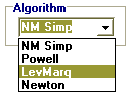
NM Simp: The modification of Nelder-Mead algorithm with “box” constrains. It is the direct search method that does not require calculation of derivatives
Powell: The modification of Powell algorithm with “box” constrains, also a direct search method
LevMarq: Levenberg-Marquard algorithm
NewtonThe combination of steepest descent method with Newton algorithm

4. Initialise the Parameters in the Circuit parameters. Constraints and results table.

Each element added to the equivalent circuit panel automatically generates default values of upper and lower limits. The default soft constraints may probably fit to most cases in electrochemical system analysis, but in many cases you may need to alter the range of expected parameter keeping in mind that the range narrowing favours the search of the solution, provided the solution falls into the range.
Three of the algorithms (Powell, LevMarq or Newton) require also initial values from which the search of the solution starts (Result/In.Val. column in the table). The closer the initial values to true values of the parameters or the narrower the range containing true value the more likely the algorithms converge fast to the global minimum. No initial value is needed for NM Simp algorithm.

5. Select the type of function to minimise.


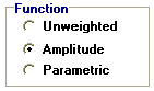
The available functions:
  
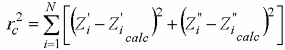
Unweighted:
r_u(ω, P₁…P_M) = r_c²/(N-M)
where N is number of points, M is number of parameters, ω is the angular frequency, P₁…P_M are the parameters and



Amplitude weighting:
r_a(ω, P₁…P_M) = r_c²/(N-M)
where



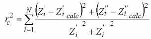
Parametric weighting:
r_p(ω, P₁…P_M) = r_c²/(N-M)
where



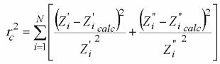
where i corresponds to measured values of impedance and i calc corresponds to the calculated values; N is a number of points.

For NM Simp and Powell algorithms, there is a possibility of setting the maximum number of iterations (on the Fitting tab control, default values are 10000 and 300 respectively).

Finally, check the working mode is Fitting and press the button (alternatively, select Model / Fit Model from the menu) to start fitting the data to the model. The progress bar and button will appear in place of Function panel.

As a result of fitting (if successful), the Result/In.Val. column of the table fills with the calculated parameters, the Error % column fills with the values of relative estimated errors of the calculated parameters, or with ###, if the element has error higher than 1000%. The calculated spectrum appears in green overlaid on the experimental spectrum. Statistics box on the Fitting page control shows normalized fitting errors in optimal solution r² = r_c²/(n-p) for complex unweighted function, for the unweighted real and imaginary parts, for amplitude weighted and for  parametric weighted, respectively. You may also see the residuals plot for modulus, real and imaginary part of impedance and also for phase shift (depending on current data plot representation) by selecting Analysis / Show Residuals. Probably you will need to press button several times repeatedly, or change the constraints and algorithm if the first attempt of finding the global minimum appears to be unsuccessful.

You may also check whether the circuit fits to a part of the spectrum by using the Fragmentary analysis mode.